Breaking New Ground: NCUM Data Modeling in SAP Datasphere vs. BW/4HANA – Part 1: Record Types
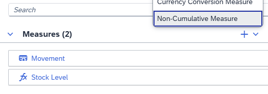
Stock and inventory data present unique challenges for reporting because they don’t aggregate over time like traditional transactional data. For example, summing up stock levels across multiple periods doesn’t yield meaningful insights since stock values depend on both historical reference points and subsequent changes. To address this, Non-Cumulative (NCUM) Key Figures are used, enabling accurate reporting by focusing on inflows and outflows rather than simple totals.
Welcome to this 4-part blog series on inventory management in BW4HANA and SAP Datasphere.
In Part 1, we’ll explore the fundamentals of inventory management within BI, focusing on key record types and providing a conceptual overview of how inventory data is structured in general.
Part 2 will dive into the non-cumulative data model in SAP BW/4HANA. Using a practical example, we’ll explain how this model works, outline its technical requirements.
Part 3 will show you a quick setup to build and understand a working NCUM environment within the SAP Datasphere (DSP) approach.
Finally, Part 4 will explore the technical steps required to achieve this functionality, including handling delta loads from an S/4HANA system.
Part 1: Record Types
When working with non-cumulative key figures in SAP BW/4HANA or SAP Datasphere, understanding record types is essential. These play a central role in enabling the system’s special aggregation behavior – but don’t worry, much of this is handled automatically by the system (in SAP BW4HANA)!
As the term suggests, a record type categorizes a data record — specifically in terms of time. In the context of inventory data, record types describe whether a value represents an inflow/outflow (no matter if in the past or future) or the current stock level.
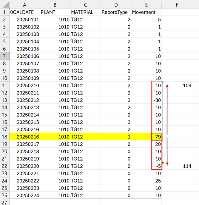
There are three main record types:
- 0 – Future Delta: Changes expected after the reference point (projected inflows/outflows).
- 1 – Reference Point: The current state or snapshot of inventory (most recent known level).
- 2 – Historical Delta: Changes that occurred before the reference point (already included in it).
To efficiently calculate inventory levels, the system typically starts from the reference point (record type 1) and then adjusts it by adding or subtracting deltas from the future (0) or the past (2).
This is far more efficient than recalculating from the very beginning of the inventory history — without a reference point, every transaction would need to be re-processed from day one to determine the current stock.
Summary
- Non-cumulative key figures (such as stock or inventory) behave differently from cumulative ones — they do not aggregate linearly over time.
- A standard summation would yield incorrect results; instead, the system applies an exception aggregation tailored for non-cumulative data.
- Record types are the technical backbone for handling this: they define whether a record reflects a change (delta, 0 or 2) or a stock level (reference point, 1), and where in time it belongs.
- By using record types, the OLAP processor can accurately position and interpret data records within the time axis — enabling correct and performant reporting for inventory use cases.