Disclaimer 

SAP recently announced the launch of SAP Datasphere, which is the next generation of SAP Data Warehouse Cloud. Therefore, also the name from SAP Data Warehouse Cloud changed to SAP Datasphere. This blog, which was posted ahead of this change, refers to SAP Data Warehouse Cloud. Everything which is mentioned within the post is also true for SAP Datasphere. 

Introduction

In the second part of our blog series, we want to analyze how Data Flows perform doing very simple tasks like we showed in the first example of our blog series (Data Flows in DWC – Part 1: Introduction). Therefore, we uploaded a 1GB CSV File to DWC and built some basic examples.

The performance will get interesting when the script operator is getting involved. But we also want to show here, how for basic tasks it could be possible to avoid the Script Operator by incorporating SQL Views and their built-in functions instead.

Setup

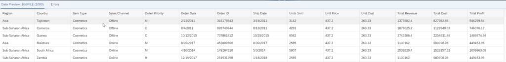
As already mentioned, we uploaded a 1GB CSV File to DWC which has 10 million records. The data contains standard Sales Data with the following columns:

• Region
• Country
• Item Type
• Sales Channel
• Order Priority
• Order Date
• Order ID
• Ship Date
• Unit Sold
• Unit Price

Performance of the “Standard Operators” in DWC

In this section we want to look at the performance of Data Flows which only contain “Standard Operators”, which we see as the following:

1. Join Operator
2. Projection Operator
3. Aggregation Operator

Example 1: Join Operator.

For this scenario we want to join based on the Region column, a Manager to a Source table.

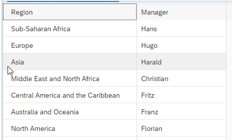
We just perform an inner join to add this information via the Join Operator.

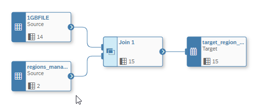
We did run this operation a couple of times and it did run around 3 minutes.

Example 2: Projection Operator Concatenation of Fields

In this example we want to concatenate two fields with the projection operator.

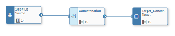
This operation ran for 2,5 minutes.

Example 3: Projection Operator and the Deletion in the target

Another Use Case we showed in the first blog post is to use the projection Operator to delete records in the target.

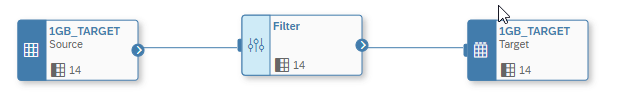
It only took ~30 seconds to perform this Data Flow.

Example 4: Aggregation Operator

The fourth example shows the runtime of the Aggregation Operator with this amount of data.

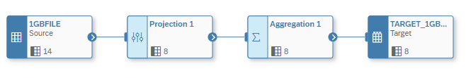
To aggregate the data into the target table the Data Flow took around 40 to 50 seconds.

Performance of the Script Operator and how you maybe need to think SQL

Within this section we want to look at how the script operator performs with this amount of data to be processed. Therefore, we decided that we want to transform the Columns “Order Date” and “Ship Date” from a character format to a date format.

The first solution did use the following Python Script with the Pandas apply function (http://pandas.pydata.org/pandas-docs/stable/reference/api/pandas.DataFrame.apply.html), applying the function to_datetime (https://pandas.pydata.org/docs/reference/api/pandas.to_datetime.html).

The script worked and transformed the column into the desired format.

However, it did run for quite some time for this simple exercise. In our system it ran for around 2 hours and 40 minutes. In comparison in a local Jupyter Notebook it took with the same coding 17 minutes.

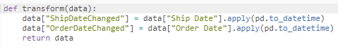
Now you might say, the apply function should be avoided as it is like a loop and that is what we did by changing our script coding to the following:

With this change we could bring down the runtime to about 47 minutes. In comparison again, this took in a local Jupyter Notebook then only 1 minute. Overall, we would like to say that this runtime is not an acceptable result for such a simple task to us.

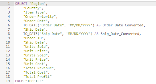
As you might know you can also build views in DWC, where you can benefit from a lot of built in functions and expressions (https://help.sap.com/docs/HANA_CLOUD_DATABASE/c1d3f60099654ecfb3fe36ac93c121bb/20a4389775191014b5a6bf2ccc0df2ed.html?locale=en-US). So, we gave it a try to perform this logic in an SQL View and include this in a Data Flow.

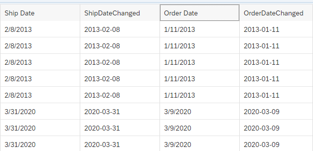
In a first step we defined a new view with the TO_DATE function.

This view we used then as a source in our Data flow and wrote it directly into the target table:

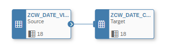
By using this approach, we could get the runtime down to about 3 minutes.

This showed us that we should think about using SQL functions whenever possible as the Script Operators performance is not good enough yet for big data amounts. But it will probably not be possible to always formulate logic in SQL, therefore it will be interesting to see how the performance will increase as the DWC will become a more mature product over time.

Conclusion

To conclude this, we want to summarize the performance results in the table below. There we can see that what we defined earlier as “Standard Operators” seem to perform quite well. In contrast the script operator did not deliver an acceptable result for us, but this easy scenario could be solved by using a SQL View without any operator being used in the Data Flow.

Scenario	Operator	Runtime
Look Up Data	Join	~3 minutes
Concatenation of Fields	Projection	~2 ½ minutes
Deletion of Records	Projection	~30 seconds
Aggregation of Data	Aggregation	~45 seconds
Transform Date String to Date (with Pandas apply function)	Script	~2 hrs and 40 minutes
Transform Date String to Date (with Pandas to_datetime function)	Script	~47 minutes
Transform Date String to Date (with SQL VIEW)	–	~3 minutes

The scenarios we have built so far are quite simple and do not contain complex logic. If we would use DWC in a productive environment we would say the “Standard Operators” you should be able to use without running into any major performance problems. However, if you use the script operator, which might be necessary at a certain point because you will not be able to transform every requirement into a SQL, you will need to check carefully your coding and how it will perform. Especially with the script operator we hope that SAP will come up with a solution that will boost the runtime.

More posts from this blog series