Introduction

In SAP Datasphere (DSP), you build Analytical Models to expose curated, business-ready data to end users. When you stay within the SAP stack, these models are most commonly consumed through SAP Analytics Cloud (SAC), where users slice, dice, and drill into the data via stories and dashboards. The closer you get to the end user, the more visible performance becomes — a query that takes 30 seconds in a developer tool feels like an eternity in a live SAC story being demoed to executives.

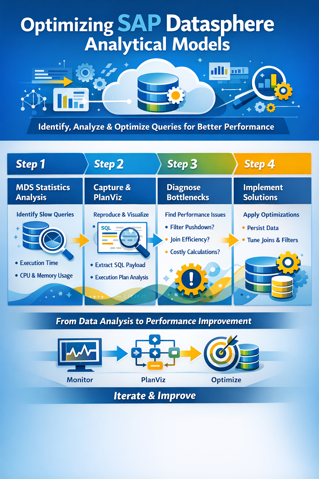
Performance tuning of Analytical Models is rarely about a single silver bullet. It’s a layered investigation: you need to know what the frontend is asking for, how the engine is executing it, where the time is spent, and which levers you can pull to improve things. Over the course of several customer projects, we’ve converged on a repeatable approach for analyzing and improving Analytical Model performance. This guide walks through that approach step by step.

Step 1 – M_MULTIDIMENSIONAL_STATEMENT_STATISTICS

The first place we always have at, is the M_MULTIDIMENSIONAL_STATEMENT_STATISTICS view (often shortened to MDS statistics). Analytical queries coming from SAC are executed as MDS (multidimensional) statements against the underlying HANA engine in Datasphere, and this monitoring view captures runtime information about each of them.

What makes this view so valuable is that it gives you a quick, high-level overview without the need to reproduce the issue yourself. You can see:

Which Analytical Model or view was queried
The total execution time
CPU time and memory consumption
The user who triggered the statement
The timestamp, so you can correlate with user complaints

A typical first query is to order by execution time descending and look at the top offenders over the last day or week. This immediately tells you whether you have a systemic problem (many models running slowly) or a localized one (one specific model dragging everything down). It also helps you separate „the model is slow“ from „the user ran a particularly nasty ad-hoc drill-down“ — both are valid performance topics, but they call for different responses.

A small caveat: MDS statistics give you the what and the how much, but not the why. To understand why a statement is slow, you need to go deeper.

Step 2 – Capture the Payload from the Frontend and Create a Plan Visualization

Once you’ve identified a problematic query, you need to reproduce it in a controlled way so you can analyze it. The trick here is that the SQL the engine executes is generated dynamically based on what the SAC story requests — the dimensions on rows and columns, the filters in the prompt, the measure selected and any user-applied filters or drill state. You can’t just guess at this; you need to capture the actual payload.

The most reliable approach is to open the browser developer tools (F12 in Chrome or Edge), switch to the Network tab, and reproduce the user action in SAC. You’ll see the request going out to Datasphere — the payload contains the analytical query in a structured form. From there, capture the resulting SQL statement that Datasphere generates and run it in a SQL console against the Datasphere space.

Once you have the SQL, generate a Plan Visualization (PlanViz) in HANA Studio or the Database Explorer. PlanViz is the single most powerful tool you have for understanding why a query is slow. It shows you the execution plan as a graph: each operator, how many rows flow in and out, how much time each step takes, and where the bottlenecks are. You’ll see joins, aggregations, filter operations, remote calls, and column scans, and you can drill into any node to inspect its details.

Without PlanViz you are guessing. With PlanViz you have evidence.

Step 3 – Identify Long-Running Tasks and Their Reasons

Armed with the execution plan, work through a checklist of common culprits. These are the questions we ask on every performance analysis:

How much data is initially selected? Look at the row counts at the leaf nodes of the plan — the table scans. If your model is supposed to return a few thousand aggregated rows, but the engine is reading hundreds of millions of records from the base tables, you have a fundamental selectivity problem. Either the filters aren’t reaching the tables, or the model is structured in a way that forces a full materialization before filtering.

Are my filters pushed down to the base tables? Filter pushdown is the single most important optimization the engine performs. A filter applied in the SAC story should ideally end up as a WHERE clause directly on the base table read. In PlanViz you can verify this by looking at the table scan nodes and checking the filter predicates. If your filter only appears way up in the plan, near the top, the engine is reading everything first and filtering afterwards — which is exactly what you want to avoid. Common reasons for failed pushdown include calculated columns referenced in the filter, certain join types, and unions over heterogeneous sources.

Are my joins correct from a business-logic standpoint? This sounds obvious, but it’s worth re-checking. An inner join versus a left outer join not only changes the result set, it changes the optimizer’s freedom to reorder and prune. Inner joins are generally easier for the optimizer to handle. Similarly, UNION versus UNION ALL matters: UNION forces a deduplication step, which is costly, and is almost never what you actually need for additive measures. Use UNION ALL whenever business semantics allow it.

Am I performing costly calculations on the fly? Calculated measures and calculated columns evaluated at query time are convenient during modeling but expensive at runtime, especially when they involve case statements, string operations, or references across joined tables. If a calculation is stable and reused often, persisting it upstream is usually a better choice than recomputing it for every query.

Are there any remote table calls? Remote tables (federated through Smart Data Integration or similar) introduce network latency and break many optimization opportunities, because the remote source may not support the same pushdown semantics. If you see remote scans in your plan and the latency dominates, the answer is almost always to replicate or snapshot the data into Datasphere rather than federate it live.

Am I reporting on tables in the Object Store? Datasphere’s object store (Data Lake) is excellent for cheap storage of large historical datasets, but query patterns matter enormously. Have you run the Merge operation to consolidate small files into larger ones? Have you run Optimize to re-cluster the data? May I need to define Z-Order columns? A model that filters on a column that isn’t in the Z-order will scan far more data than necessary.

Step 4 – Think About Solutions

Once you understand the bottleneck, the next question is what to do about it. There is rarely one right answer; the right answer depends on data volume, refresh frequency, latency requirements, and cost. Here are the levers we reach for most often.

Persisting views. Datasphere allows you to persist the result of a view, materializing it on a schedule. For views that sit on top of complex joins or expensive calculations and don’t need to be real-time, this is an enormous win. The end-user query then reads from a flat persisted table instead of re-executing the entire transformation graph each time.

Locked partitions. When persisting large views, you can use locked partitions to refresh only a subset of the data — typically the most recent slice — while leaving historical partitions untouched. This dramatically reduces the cost and runtime of the refresh job and makes large persisted views actually viable.

Persist logic via local tables and transformation flows. For more complex pipelines, instead of layering view on view on view, you can write the intermediate results into local tables using transformation flows. This gives you full control over scheduling, partitioning, and incremental loads, and it shortens the runtime path of the consuming query.

Push filters via joins and input parameters. When filter pushdown isn’t happening naturally, you can sometimes force it by introducing input parameters that are used directly in the lower layers of the model, or by restructuring joins so that filtered data flows into the join rather than being filtered after the join. Input parameters in particular are useful when the model is consumed with mandatory prompts in SAC: the parameter value reaches the base table directly.

Additional Steps

Beyond the main loop above, there are several supporting investigations and tools that frequently come into play:

Check the system logs. Datasphere exposes logs for task execution, persistence runs, and remote source connectivity. If a model is intermittently slow, the explanation is often hiding in a failed or retried background job rather than in the query itself.

Check the HANA Cockpit for detailed analysis and OOM diagnostics. When queries fail outright with out-of-memory errors, the HANA Cockpit gives you the detailed memory consumption breakdown, the offending statement, and often a root-cause hint. OOM situations are usually a symptom of unbounded intermediate result sets — large unfiltered joins, missing aggregations or runaway cross products — and the cockpit is the fastest way to pinpoint which.

Think about workload classes. Workload classes let you assign resource limits and priorities to different categories of queries or users. This won’t make a slow query fast, but it will prevent one heavy user from monopolizing resources and degrading everyone else’s experience. For mixed workloads — interactive SAC users alongside batch persistence jobs — workload classes are essential for predictable performance.

Evaluate elastic compute nodes. For workloads that are spiky (month-end close, quarterly reporting, big planning runs), elastic compute nodes let you temporarily add capacity without permanently scaling up your tenant. They’re particularly useful when the bottleneck is genuinely compute-bound rather than model-design-bound — but be honest with yourself about which one it actually is, because throwing hardware at a badly modeled view is expensive and only partially effective.

Closing Thoughts

Performance tuning of Analytical Models in Datasphere is an iterative discipline. Start with the evidence (M_MULTIDIMENSIONAL_STATEMENT_STATISTICS), reproduce the problem with the real frontend payload, analyze the execution plan, and only then reach for solutions. Resist the temptation to persist everything by default — persistence has its own cost in terms of refresh windows, storage, and data freshness — and resist the temptation to scale up before you’ve understood the model. The biggest wins almost always come from fixing pushdown, simplifying joins, and persisting the right layer at the right grain. Hardware and workload management are there to handle what’s left over.